hcphases turns a homological quantum-code model into a numerical experiment: define the geometry and couplings, choose observables, then sample a classical system representing its thermal state. I developed it as part of my work on topological phases and quantum information.
The package supports local Pauli operators, extended Wilson and ’t Hooft operators, selected decoded observables, products and connected correlations. It also retains measurement histories, diagnostics and software identities, so a result can be traced back to the calculation that produced it. The repository and documentation are the starting points for using it.
The quantum models
Place qubits on the \(p\)-dimensional cells of a periodic \(d\)-dimensional cubical lattice: edges for \(p=1\), faces for \(p=2\), and so on. Two families of commuting stabilizers describe the code. \(A_a\) multiplies Pauli \(X\) operators on the cells incident on a \((p-1)\)-cell; \(B_b\) multiplies Pauli \(Z\) operators around the boundary of a \((p+1)\)-cell. Uniform fields perturb the code Hamiltonian:
\[\begin{aligned} H={}&-\frac{J}{2}\sum_a(1+A_a) \\ &-\frac{K}{2}\sum_b(1+B_b) \\ &-g\sum_e X_e-h\sum_e Z_e. \end{aligned}\]
For positive \(J,K\), the zero-field ground space is the code space. At temperature \(T\), the target is the full Gibbs state \(\rho=e^{-H/T}/\mathrm{Tr}(e^{-H/T})\), including excitations and all logical sectors. The implemented samplers cover binary codes with \(d\geq2\), \(1\leq p<d\), and a separate one-dimensional vertex model. The model reference fixes the conventions; the support matrix gives the allowed parameters.
A classical equilibrium measure
Split \(H=H_z+H_x\) into its diagonal and spin-flip parts. With \(M\) imaginary-time slices and \(\delta=1/(TM)\), the package represents the ordered trace \(Z_M=\mathrm{Tr}[(e^{-\delta H_z}e^{-\delta H_x})^M]\). This becomes a sum over binary configurations \(\phi\) on a periodic spacetime lattice, with equilibrium probability
\[\pi_M(\phi)=\frac{w_M(\phi)}{\sum_{\phi'}w_M(\phi')}.\]
Write \(\sigma_e=(-1)^{\phi_e}\) for a spin on a spacetime cell and \(P_f=\prod_{e\in\partial f}\sigma_e\) for the spin product around a cell boundary. Up to a configuration-independent factor, the Boltzmann weight is \(w_M\propto e^{S_M}\), with
\[\begin{aligned} S_M={}&\kappa_s\sum_{f_s}P_{f_s}+\kappa_t\sum_{f_t}P_{f_t} \\ &+h_s\sum_{e_s}\sigma_{e_s}+h_t\sum_{e_t}\sigma_{e_t}. \end{aligned}\]
The subscripts distinguish spatial and temporal cells. These four dimensionless couplings are determined by \(J,K,g,h\) and \(\delta\). For the supported sampling parameters the weights are positive. Quantum observables become classical estimators; \(X\)-type measurements use a separate dual ensemble with exchanged couplings.
This mapping is exact for the chosen finite-\(M\) transfer product. Recovering the quantum Gibbs state requires convergence as \(M\) increases at fixed Hamiltonian and temperature. The measure and couplings are documented separately.
Sampling, including the logical sectors
For higher-degree codes, the sampler combines local Metropolis flips with worldline proposals that flip a spatial cell across every time slice. For the vertex model, it uses a Wolff-style cluster update: connected groups of aligned spins flip together. Measurements follow a fixed number of attempted updates, including deliberately idle steps.
Topology needs extra care. Noncontractible logical shifts can be difficult to explore using local moves alone. The higher-degree engine sums over the spatial coordinate logical shifts analytically, with their actual conditional weights, and samples the remaining background. Observables receive the matching conditional average; treating sectors as equally weighted or measuring an unaveraged operator would generally give the wrong answer.
This removes the need for the chain to tunnel between those particular logical shifts. It does not guarantee equilibration of the remaining background, or compute all separate sector partition functions. The vertex demo below samples the ordinary periodic Ising ensemble; it does not average over boundary twists. See the logical-sector treatment and sampling algorithms for the details.
Code in action: the 2D Ising model
The simplest demonstration starts with a quantum chain:
\[\begin{aligned}H={}&-\frac K2\sum_j(1+Z_jZ_{j+1}) \\ &-g\sum_jX_j.\end{aligned}\]
Its classical image is the two-dimensional Ising model, with one spatial and one imaginary-time direction. The dimensionless couplings are \(\kappa_x=\delta K/2\) and \(\kappa_\tau=-\tfrac12\log\tanh(\delta g)\). Setting \(L=M=n\), \(T=1/n\), \(K=2\kappa\) and \(g=-\log(\tanh\kappa)/2\) makes both couplings equal.
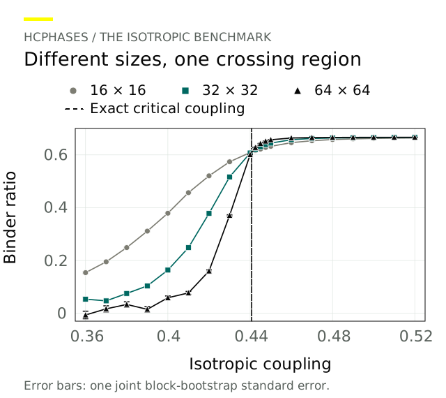
To distinguish ordered and disordered behavior, we measure the magnetization per spin, \(m=(LM)^{-1}\sum_{j,t}\sigma_{j,t}\), and its second and fourth moments. These define the dimensionless Binder ratio (also called the Binder cumulant):
\[U_4=1-\frac{\langle m^4\rangle}{3\langle m^2\rangle^2}.\]
The brackets denote equilibrium averages. This ratio describes the shape of the magnetization distribution: it approaches zero deep in the disordered phase and \(2/3\) deep in the ordered phase of the zero-field Ising model as the system becomes large. Curves for different lattice sizes cross near the transition, providing a finite-size estimate of the phase boundary. The original Binder reference and the benchmark report give the details.
Here is a compact one-point example: declare the model, measure the two moments, and combine their pooled means into \(U_4\). Use a fresh output directory with Python 3.12; the current bounded runner uses Windows. These short settings illustrate the API, rather than reproduce the full scan.
from math import log, tanh
from hcphases import (
    VertexModel, VertexObservable, VertexSamplingPlan,
    ResourceBudget, run_vertex, read_vertex_records,
)

def main():
    n, kappa = 16, 0.44
    model = VertexModel(
        length=n, slices=n, T=1/n,
        K=2*kappa, g=-log(tanh(kappa))/2,
    )
    observables = {
        "m2": VertexObservable(kind="magnetization", power=2),
        "m4": VertexObservable(kind="magnetization", power=4),
    }
    receipt = run_vertex(
        model, observables, seed=12345, output="ising-demo",
        sampling=VertexSamplingPlan(
            chains=2, starts=("ordered", "hot"),
            warmup_steps=256, sample_steps=1024, measure_every=4,
        ),
        resources=ResourceBudget(
            wall_seconds=60, memory_bytes=2**30,
            output_bytes=32*2**20,
        ),
    )
    if receipt["terminal_reason"] != "completed":
        raise RuntimeError(receipt)
    metadata, samples = read_vertex_records("ising-demo")
    columns = metadata["columns"]
    m2 = samples[:, :, columns.index("m2")].mean()
    m4 = samples[:, :, columns.index("m4")].mean()
    binder = 1 - m4 / (3 * m2**2) if m2 > 0 else None
    print(binder)

if __name__ == "__main__":
    main()
In the saved scans, comparing Binder curves for sizes 16, 32 and 64 locates the transition. The 32/64 isotropic crossing is 0.44113, versus the exact 0.44069, a difference of 0.10%. Varying the two couplings independently gives the phase boundary below; the exact line satisfies \(\sinh(2\kappa_x)\sinh(2\kappa_\tau)=1\).
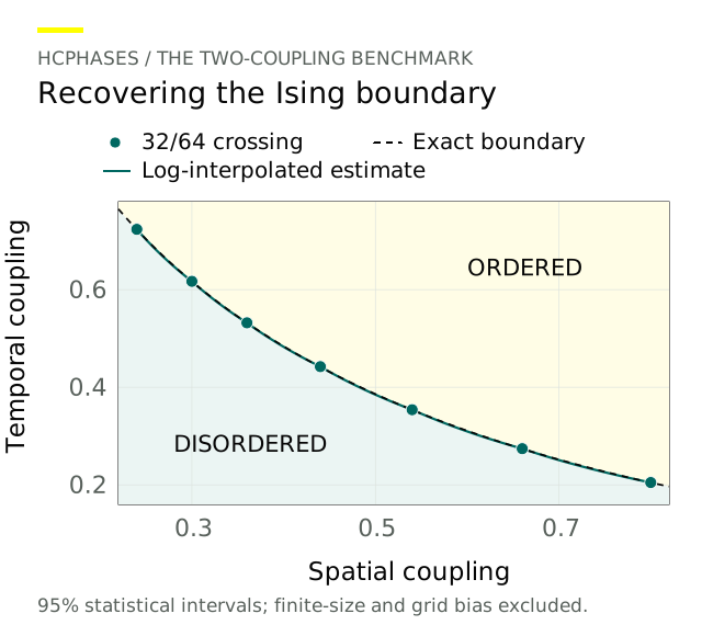
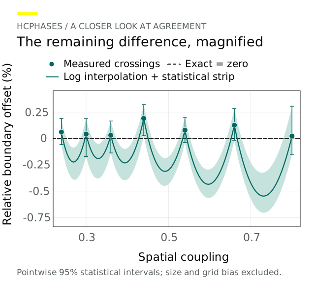
The seven measured crossings deviate from the exact line by at most 0.191%; interpolation between them reaches 0.546% on the comparison grid. These are finite-size classical benchmarks. Statistical intervals exclude size and grid bias—in particular, the isotropic exact value lies outside its statistical-only 95% interval. Inspect the Binder curves and boundary residuals in the supplementary figures below, or open the full report (PDF). The quickstart adds audits and sampling diagnostics to the example above.
This familiar model gives a first check of the workflow. The same framework supports studies of other code geometries, observables and phase boundaries.
Supplementary figureBinder curves: locating the transition
Supplementary figureBoundary residuals: resolving the differences